Exploring 2014 Denver B-cycle Ridership

Denver, Colorado is considered to be one of the most bikeable cities in America. In addition to the fine bike lanes, bike trails, and mostly favorable weather (300 days of sunshine, says the possibly dubious but sunny claim), Denver is also a B-cycle city, with bicycle rental kiosks dotting the sidewalks near the city center. For this short study, I obtained Denver’s 2014 B-cycle trip data, and used it along with some other data sources to see if I could model hourly ridership across the Denver B-cycle network. My study indicated that most calendar and clock variables are highly significant when predicting ridership, and weather variables such as temperature and amount of cloud cover appear to be as well. This post details how I obtained the data, how I merged data from different sources, shows some explorations of the data, and finally shows how I created a regression model of system ridership.

About B-cycle

B-cycle is a public bicycle sharing company that operates in several cites, including Denver, Colorado. The premise is that users may “checkout” a bike from a kiosk, which is usually along a city sidewalk, under various short- to long-term access passes, depending on the user’s preference and anticipated usage. In Denver, most of the kiosks appear to have 10-20 “docks” where the bikes are stored until a user checks out the bike. After a user checks out a bike, they ride it for as long as they wish, and then check it back in any B-cycle kiosk. In 2014, Denver B-cycle operated 84 different kiosks, which are mostly clustered around the city center. At the end of the year, B-cycle posts their yearly trip data as an Excel spreadsheet on their company webpage. I used these data, along with data from a few other sources, to conduct this study. For more information, please see the Denver B-cycle homepage.

Data Acquisition and Merging

For this report, I obtained data from several sources and combined the data together, taking the following steps. Most of the initial data download and munging steps can be replicated by looking at the exploring_bcycle_data.Rmd file; most of these steps were too time-intensive to be carried out in a production-level script.

1. Downloaded B-cycle 2014 Trip Data from the B-Cycle company information webpage. I did some date munging and changed variable names to ones that are more R-friendly.
2. Obtained B-cycle kiosk data (kiosk name and address) by hand from the Denver B-cycle homepage.
3. Created a list of the 6800 combinations of checkout kiosk/return kiosk. For each combination, I used the mapdist function from R’s ggmap package to find the approximate bicycling distance and time between each kiosk. Because of the large number of one-way streets in the Denver downtown area, where the kiosks are highly clustered, I chose to find each checkout-return pair’s distance separately, rather than finding a single distance for each pair regardless of direction of travel. This process took three days, because the Google Distance Matrix API (which the mapdist function uses) only allows 2500 calls a day.
4. Found the latitude and longitude for each station using the geocode function in the ggmap package.
5. Obtained an API key from forecast.io. Within R, in my exploratory Rmd file, I wrote a function to download the weather data from forecast.io. Each day’s hourly data comes in a separate JSON file; I saved each JSON file to a directory.
6. Within the production script, I merged different parts of the above data in different ways, depending on the specific task goals. The final merging was to merge aggregated hourly checkout data with the hourly weather data.

A Note about Holidays

For my study, I factored in City of Denver observed holidays. Denver city celebrates all the same holidays as the federal holidays, with the following exception: Columbus Day is not a city holiday, and is replaced by Cesar Chavez Day, usually in late March. I only factored in the major federal holidays that result in government and bank closures (with the exception above), and not the lesser holidays.

Basic Ridership Statistics

Number of Rides

The B-cycle data, as downloaded, contains 377,229 rows of “trip data.” Nominally, this means that 377,229 B-cycle trips were taken in 2014. Indeed, the 2014 Denver B-cycle annual report claims this to be the number of rides for the year.

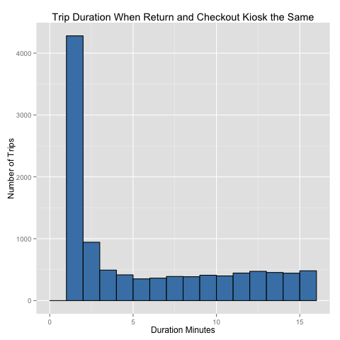
However, over 1% of the rides (4279 rides) have the same checkout station as return station with a trip duration of only 1 minute (see Figure 1 below). I believe these should be filtered out because I believe the majority of these “rides” are likely people checking out a bike, and then deciding after a very short time that this particular bike doesn’t work for them. I believe that most of the same-kiosk rides under 5 minutes or so likely shouldn’t count, but only culled the ones that were one minute long.

I also filtered out 258 rides with an “invalid return” station. This could be any number of things, but since finding nominal distance for these rides is very difficult, I filtered these out as well.

With the above, I arrived at an estimate of 372,684 B-cycle rides in 2014.

Distance Traveled

As mentioned in bullet #3 in the Data Acquisition section, I used a Google Maps API in the ggmap package to derive the between-station distance for each station pair and then for each ride. Because a large number of rides were returning to the same kiosk, meaning the minimum distance ridden cannot be estimated by Google Maps, I estimated the distance ridden by calculating the average speed of all the other rides (nominal distance ridden divided by the duration), and then applying this average speed to the same-kiosk trip durations, capping the trips at an arbitrary 5 miles. While it’s likely I am underestimating the total distance ridden by a fair amount (perhaps 25%), since many riders will not take the straight-line distance between two stations (especially tourists/non-commuters), I estimate riders rode at least 616,960 miles on B-cycle in 2014, with a more likely number 25% higher at 771,200 miles.

Most Popular and Least Popular Kiosks

Most Popular

The following ten kiosks are the most popular kiosks by number of total bike checkouts in 2014. The return kiosk popularity is very similar.

REI                     9898
14th & Stout            8903
22nd & Market           8896 
18th & California       8363
1350 Larimer            8273
13th & Speer            8128
Market Street Station   8116
1550 Glenarm            7940
16th & Platte           7714
Denver Public Library   7401

Least Popular

The following ten kiosks are the least popular kiosks by number of total bike checkouts in 2014.

29th & Zuni                      780
Florida & S. Pearl               987
Louisiana / Pearl Light Rail    1407 
Ellsworth & Madison             1523
Pepsi Center                    1610
Denver Zoo                      1704
33rd & Arapahoe                 1851
32nd & Juliann                  1926
Colfax & Garfield               1989
32nd & Clay                     1997

Map of Station Popularity

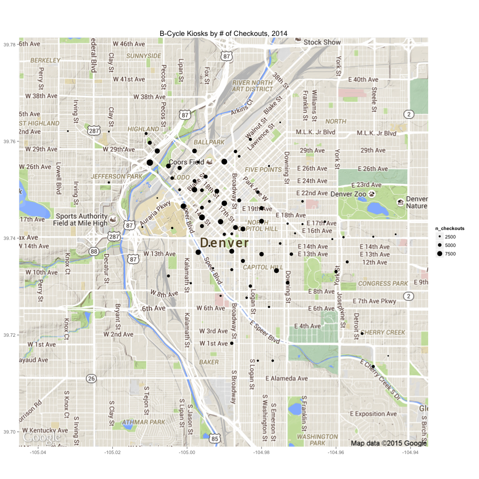
I used the ggmap package to create the following map showing the popularity of the various checkout kiosks (Figure 2). The size of the circle is proportional to the number of checkouts from that kiosk in 2014.

Checkouts Per Membership Type

B-cycle has a number of different membership passes. The following were the top 5 by number of checkouts in 2014.

Annual (Denver Bike Sharing)               232180                                  
24-hour Kiosk Only (Denver Bike Sharing)   119489                    
30-day (Denver Bike Sharing)                 6025
Not Applicable                               4490
7-day (Denver Bike Sharing)                  3853 

Ridership by Calendar and Clock Variables

Ridership by Hour

To dive a little deeper into the data, I aggregated the data by taking the total number of bike checkouts for each hour of the year. All checkouts in a given hour were assigned to that specific hour (i.e. a checkout at 6:02 AM and a checkout at 6:56 AM both count as a checkout in the 6 AM hour).

I then totaled the number of checkouts in a given hour of the day – summing up over the entire year (so the 10 AM sum is the total number of riders checking out a bike in the 10 AM hour for the 365 days in 2014). Figure 3 below shows the total number of bike checkouts for each hour of the day, and Figure 4 shows the estimated distance ridden given the hour of checkout.

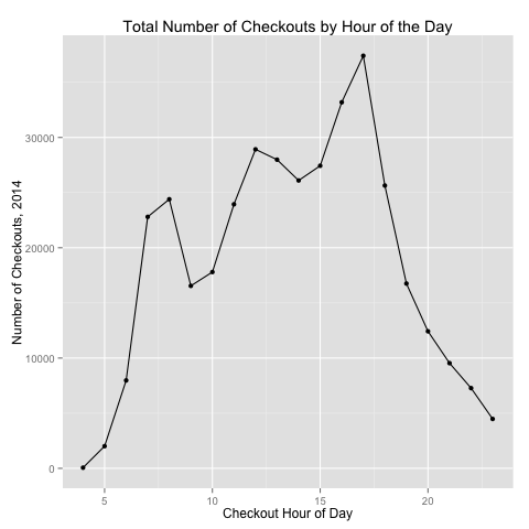
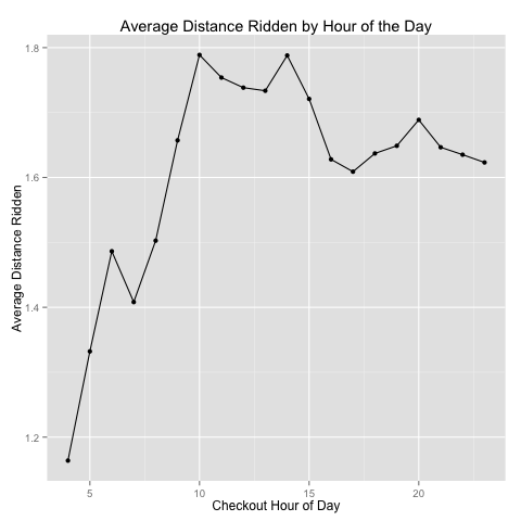
These figures show that most bike checkouts occur during the 4 PM and 5 PM hours, likely for the evening commute; however, people are more likely to ride a longer distance during the middle of the day – this may have more to do with the “tourist factor.”

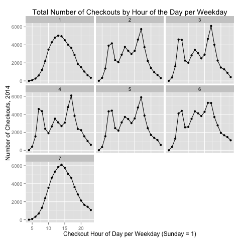
Ridership by Hour and Weekday

I also looked to see if the above patterns held true each day of the week, or if the patterns were perhaps different on the weekend. Indeed, as Figure 5 below shows, the weekday patterns (days 2-6) are all fairly similar; the weekend patterns show a significantly different shape, with usage peaks occuring between 1 PM and 3 PM.

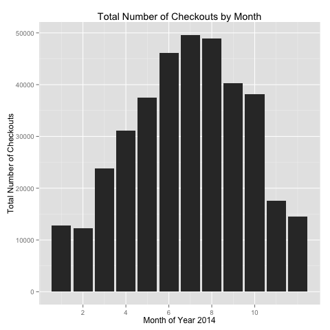
Ridership by Month

Another calendar factor I explored was the number of checkouts by month. Unsurprisingly, as Figure 6 shows, most bike checkouts occur during the summer months of June through August, and the fewest checkouts occur during the winter.

Merging with Weather

After looking at ridership as it relates to calendar and clock variables, I merged the data with hourly historical weather data. My hypothesis, based on observations of bicycle riding around Denver, is that in addition to ridership being affected by the time of day, ridership is also affected by the weather. We would likely expect more riders on warmer days (the monthly ridership statistics may be a proxy for this).

Checkouts vs. Temperature

One variable I plotted is the number of bike checkouts versus the temperature (Figure 7 below). I noted that the relationship between numbers of riders and temperature appeared to follow curve, rather than just a straight line. I fit a loess curve in ggplot to visualize the curve; based on this, in my linear regression in the next section, I used temperature and temperature squared for my linear model fit.

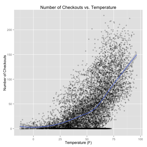
In my linear model, I also considered humidity levels and cloud cover levels.

Days with Highest/Lowest Ridership

I also found the 10 days with the highest total number of rides, as well as the 10 days with the fewest number of rides. See tables below. Unsurprisingly, the days with highest ridership were mostly warm (but not overly hot) weekend days, and the days with the least ridership were cold weekend days. One reason for this effect may be that people who commute to/from work via B-cycle may be less affected by the weather in their decision to ride, while the “weekend warriors” who rent the B-cycles for pleasure are highly affected by the weather in their decision to ride.

Highest Ridership Days

[1] "Top 5 Days by Total Number of Checkouts:"
Source: local data frame [10 x 5]

         date total_checkouts max_temp min_temp   weekday
1  2014-07-19            2181    91.96    61.79  Saturday
2  2014-08-01            2085    78.98    56.26    Friday
3  2014-07-05            2082    90.78    61.51  Saturday
4  2014-06-25            2064    84.34    56.20 Wednesday
5  2014-08-02            2027    81.67    54.46  Saturday
6  2014-07-03            1950    89.01    57.01  Thursday
7  2014-07-18            1917    85.38    59.38    Friday
8  2014-07-25            1914    90.50    67.80    Friday
9  2014-07-10            1892    91.93    62.38  Thursday
10 2014-10-04            1892    71.55    39.93  Saturday

Lowest Ridership Days

[1] "Top 5 Days by Fewest Number of Checkouts:"
Source: local data frame [10 x 5]

         date total_checkouts max_temp min_temp  weekday
1  2014-01-05              25     9.21    -2.79   Sunday
2  2014-01-04              30    39.38     9.79 Saturday
3  2014-02-01              40    24.57    11.21 Saturday
4  2014-12-26              42    19.33     9.12   Friday
5  2014-12-30              44     1.49   -10.55  Tuesday
6  2014-05-11              60    46.47    32.10   Sunday
7  2014-11-15              64    23.64     6.78 Saturday
8  2014-12-27              67    27.17     4.78 Saturday
9  2014-12-29              69    18.00     1.94   Monday
10 2014-04-13              75    46.68    20.79   Sunday

Linear Model

My final task in this short study was to attempt to create a linear regression model using a number of calendar variables and weather variables.

Setting Up Input Variables

To create this model, I forced the calendar variables to be “factor” variables. For example, it makes little sense to treat the months as actual integers – the integers denoting the months are stand-ins for the months’ names. Similarly, because peoples’ schedules do not follow a linear trajectory throughout the day, despite the increasing hours (the activity levels are more sinusoidal), it makes more sense to treat hour variables as individual factors. Likewise for weekday factors. I also have holiday factors – either 1 for holiday or 0 for not a holiday.

For the weather variables, I have temperature and temperature squared, since the ridership vs. temperature is not a straight linear relationship. I also used humidity (values between 0 and 1.0), and cloud cover (values between 0 and 1.0).

Model Output

Using the above inputs, I created a linear model. A summary of the linear fit shows the following output. An interpretation follows in the next section.

fol <- formula(num_checkouts ~ temperature + temp_sq + humidity + month + wday + hour + is_holiday + cloud_cover)
                        
Call:
lm(formula = fol, data = merged_data)

Residuals:
   Min     1Q Median     3Q    Max 
-83.76 -14.02  -1.27  12.56 148.12 

Coefficients:
              Estimate Std. Error t value Pr(>|t|)    
(Intercept) -2.833e+01  2.561e+00 -11.060  < 2e-16 ***
temperature -4.677e-01  5.315e-02  -8.800  < 2e-16 ***
temp_sq      1.789e-02  6.025e-04  29.698  < 2e-16 ***
humidity    -4.332e-01  1.919e+00  -0.226  0.82141    
month2       1.115e+00  1.278e+00   0.872  0.38303    
month3       8.045e+00  1.257e+00   6.399 1.64e-10 ***
month4       1.036e+01  1.346e+00   7.698 1.53e-14 ***
month5       6.819e+00  1.545e+00   4.415 1.02e-05 ***
month6       3.727e+00  1.778e+00   2.096  0.03612 *  
month7      -4.154e+00  2.014e+00  -2.062  0.03921 *  
month8       1.857e+00  1.892e+00   0.981  0.32639    
month9       1.061e+00  1.752e+00   0.606  0.54460    
month10      1.167e+01  1.441e+00   8.101 6.21e-16 ***
month11      2.439e+00  1.259e+00   1.937  0.05274 .  
month12      3.514e+00  1.251e+00   2.809  0.00499 ** 
wday2        4.448e+00  9.715e-01   4.578 4.75e-06 ***
wday3        4.379e+00  9.582e-01   4.570 4.95e-06 ***
wday4        4.718e+00  9.500e-01   4.966 6.95e-07 ***
wday5        6.542e+00  9.556e-01   6.846 8.10e-12 ***
wday6        9.304e+00  9.545e-01   9.747  < 2e-16 ***
wday7        8.487e+00  9.532e-01   8.904  < 2e-16 ***
hour1        3.736e-01  1.766e+00   0.212  0.83249    
hour2        1.406e+00  1.763e+00   0.797  0.42523    
hour3        2.405e+00  1.761e+00   1.366  0.17212    
hour4        2.846e+00  1.770e+00   1.608  0.10784    
hour5        9.176e+00  1.764e+00   5.203 2.00e-07 ***
hour6        2.611e+01  1.763e+00  14.812  < 2e-16 ***
hour7        6.521e+01  1.766e+00  36.916  < 2e-16 ***
hour8        6.601e+01  1.761e+00  37.491  < 2e-16 ***
hour9        3.927e+01  1.766e+00  22.240  < 2e-16 ***
hour10       3.693e+01  1.777e+00  20.783  < 2e-16 ***
hour11       4.943e+01  1.790e+00  27.623  < 2e-16 ***
hour12       5.910e+01  1.805e+00  32.739  < 2e-16 ***
hour13       5.335e+01  1.815e+00  29.388  < 2e-16 ***
hour14       4.746e+01  1.822e+00  26.044  < 2e-16 ***
hour15       5.116e+01  1.827e+00  28.009  < 2e-16 ***
hour16       6.745e+01  1.817e+00  37.126  < 2e-16 ***
hour17       8.211e+01  1.804e+00  45.514  < 2e-16 ***
hour18       5.358e+01  1.795e+00  29.849  < 2e-16 ***
hour19       3.255e+01  1.781e+00  18.272  < 2e-16 ***
hour20       2.549e+01  1.768e+00  14.412  < 2e-16 ***
hour21       2.122e+01  1.767e+00  12.012  < 2e-16 ***
hour22       1.628e+01  1.766e+00   9.218  < 2e-16 ***
hour23       1.077e+01  1.761e+00   6.112 1.02e-09 ***
is_holiday  -2.896e+00  1.536e+00  -1.885  0.05944 .  
cloud_cover -4.018e+00  1.230e+00  -3.267  0.00109 ** 
---
Signif. codes:  0 ‘***’ 0.001 ‘**’ 0.01 ‘*’ 0.05 ‘.’ 0.1 ‘ ’ 1

Residual standard error: 23.78 on 8714 degrees of freedom
Multiple R-squared:  0.7382,	Adjusted R-squared:  0.7368 
F-statistic:   546 on 45 and 8714 DF,  p-value: < 2.2e-16

Model Findings

I have a few intepretations of the above model:

• The R-squared statistic of 0.7382 means that approximately 73.8% of the variation in the hourly ridership can be explained by the chosen variables and model.
• The residual standard error of 23.78 means that, for each hour, about 2/3 of the time the model will predict total system ridership within plus or minus 23.78 riders.
• Most of the calendar variables are highly significant predictors:
  • All of the hours of the day from 5 AM onward are significant.
  • All days of the week are significant predictors.
  • Roughly half of the months are significant predictors.
  • Holidays are weakly significant predictors. This isn’t surprising, since holidays aren’t one typical unit. For instance, there may be lower ridership on “family holidays” such as Christmas and Thanksgiving than there are for holidays where people are more out-and-about, such as July 4th and Memorial Day, no matter the weather conditions.
• Some weather variables are significant, others are not:
  • Temperature and temperature squared are both highly significant predictors.
  • Humidity is not a significant predictor of ridership.
  • Proportion of cloud cover appears to be a signifant predictor, with a negative slope. That is, a fully cloudy day will have, on average, 4 few riders per hour than an otherwise identical day that is fully sunny.

Summary

Based on my short study of 2014 Denver B-cycle trip data, I found that we can create a linear model of trip ridership based on several calendar and clock variables merged with basic weather data. My study focused on total system ridership, on an hourly basis, rather than modeling specific checkout or return kiosks. Most calendar variables are highly significant when predicting ridership, and weather variables such as temperature and amount of cloud cover appear to be as well. Based on R-squared, approximately 73.8% of the variation in hourly ridership can be explained by the simple model.

Additional Areas of Study

I have many more ideas of ways that we could study this data, which I did not have time for in this particular project. The following are some of these ideas:

• Graph analysis – Which checkout/return kiosk routes most heavily used
• Kiosk predictive analytics – How to optimize the distribution of bikes at kiosks to make sure there are enough?
• Find a better method of predicting distances ridden.
• Trend analysis of ridership over more years than just 2014 – how is the program growing, and can we predict its growth in the near future?
• Break down hourly data into 15-minute increments for finer-grain resolution of ridership data – do we see a spike just before or just after the top of the hour during commuting times?
• Use autoregressive weather variables (like “lagged” temperature variables). Perhaps people may be less likely to use a B-cycle today if yesterday was very cold (even if today’s a bit warmer – but perhaps the opposite is true!).
• Model “interactions” between variables in the linear model. As it is, the variables are being modeled individually; however, there are likely significant interactions between variables that we should model (for instance, 75 degrees at 10 AM is different than 75 degrees at 9 PM with respect to ridership).
• Actually use some machine learning techniques to see if we can produce better predictions than the linear model, and test with training/validation/testing sets. I believe that if we tested some decision-tree methods (such as random forests or gbms), that we could likely get much higher predictive power than the linear model can give us.

About this Project, Source Code

I originally completed this project in August 2015 as my final project for University of Washington’s Methods for Data Analysis class, course #2 of 3 in the Data Science Certificate program. This blog post has only been slightly modified from my assignment submission. Source code for the analysis, in addition to other project files and data, can be found in my denver_bcycle repo on GitHub.